Test MITgcm

Test MITgcm using barotropic and baroclinic gyros

Compile the code

Compile the barotropic tutorial cases without OpenMPI:

cd $MITGCM_DIR/verification/tutorial_barotropic_gyre/build/
../../../tools/genmake2 "-mods" "../code"
make depend
make

Compile the baroclinic tutorial cases using OpenMPI:

cd $MITGCM_DIR/verification/tutorial_baroclinic_gyre/build/
cp ../code/SIZE.h ../code/SIZE.h_save
cp ../code/SIZE.h_mpi ../code/SIZE.h
../../../tools/genmake2 "-mpi" "-mods" "../code" "-optfile" "/home/cpapadop/MITGCM_WRF/sio_build_options/ring_build_pgi_17.5-0_openmpi_2.1.1_netcdf.3.6.3"
make depend
make

The MITGCM_DIR is the location of MITgcm source code. When compiling MITgcm, the source code in ../code/ folder will be copied to the ./build/ folder. The utility genmakes will generate the Makefile of MITgcm and utility make will compile MITgcm. If MITgcm is compiled successfully, the executable file mitgcmuv can be seen in the build folders of both cases.

Run the code

Before running the code, the input conditions/setup are required:

# After the code is compiled in the "build" folder
cd  ../run/
ln -s ../input/* .
ln -s ../build/mitgcmuv .

For the gyro_barotropic case, it is compiled without OpenMPI and should run in serial:

./mitgcmuv

For the gyro_baroclinic case, it is compiled using OpenMPI and should run in parallel:

mpirun -np 4 mitgcmuv

Post-processing

First, add the path of the matlab post-processing code to the matlab path (in MATLAB):

addpath('$MITGCM_DIR/utils/matlab/')

Using the matlab code that MITgcm provided with us:

U=rdmds('U');
V=rdmds('V');
XG=rdmds('XG');
YG=rdmds('YG');
contourf(XG,YG,U(:,:))
contourf(XG,YG,V(:,:))
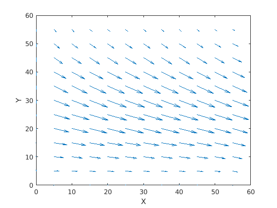
quiver(XG(1:5:end,1:5:end),YG(1:5:end,1:5:end),U(1:5:end,1:5:end),V(1:5:end,1:5:end))

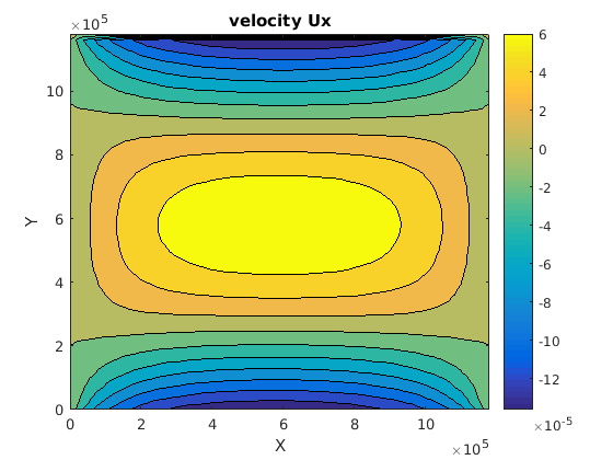
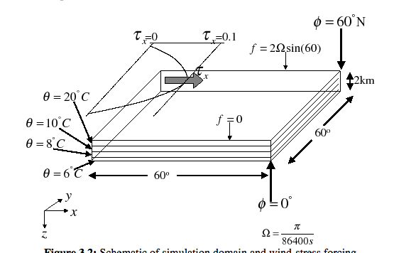
Then, we can obtain the contours of the flow velocity obtained in the gyro_barotropic case. The setup of the barotropic gyro is:

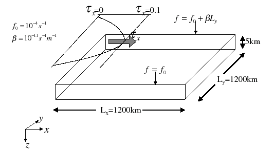
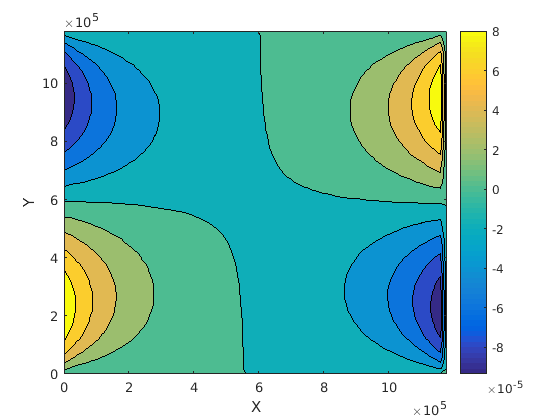
Contour of flow velocity (Ux)	Contour of flow velocity (Uy)
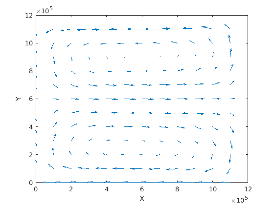
Quiver plot of flow velocity

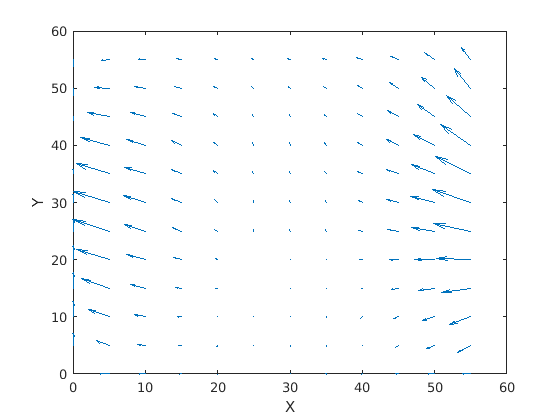
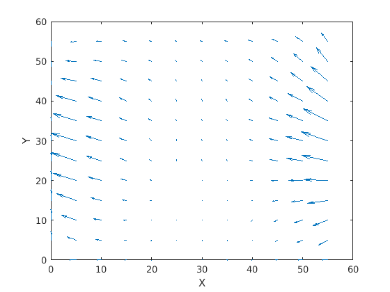
The setup of the baroclinic gyro is:

The quiver plot of the flow velocity are:

Flow velocity at Z = Z0	Flow velocity at Z = Z1
Flow velocity at Z = Z0	Flow velocity at Z = Z1

Python can also do the post-processing of the MITgcm results (need to install MITgcmutils in the MITgcm code):

cd $MITGCM_DIR/utils/python/MITgcmutils/
python setup.py install --user

To plot the MITgcm results using python:

import MITgcmutils
import matplotlib.pyplot as plt

meshX = MITgcmutils.rdmds('$MITGCM_RESULTS_DIR/XC')
meshY = MITgcmutils.rdmds('$MITGCM_RESULTS_DIR/YC')
results = MITgcmutils.rdmds('$MITGCM_RESULTS_DIR/U')
plt.contourf(mitgcm_meshX,mitgcm_meshY,results[0,:,:])

Test MITgcm using global case

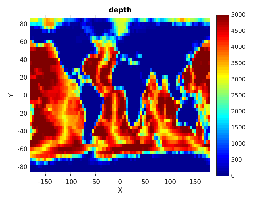
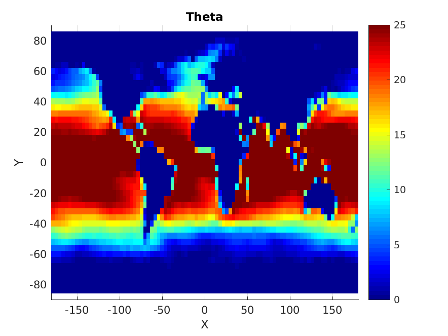
This is an MITgcm test case global_ocean.cs32x15 of 4x4 global simulation with seasonal forcing. (The mesh resolution is Nx*Ny = 90x40 in both directions.)

The input surface fluxes are from the monthly means of the NCEP climatology, including the wind stress, heat flux, salinity flux, e.t.c.

Currently the results from the MITgcm solver and MITgcm—ESMF coupled solver are identical because the coupled solver does not provide “new” information on the input values.

Depth of the ocean	Sea Surface Temperature
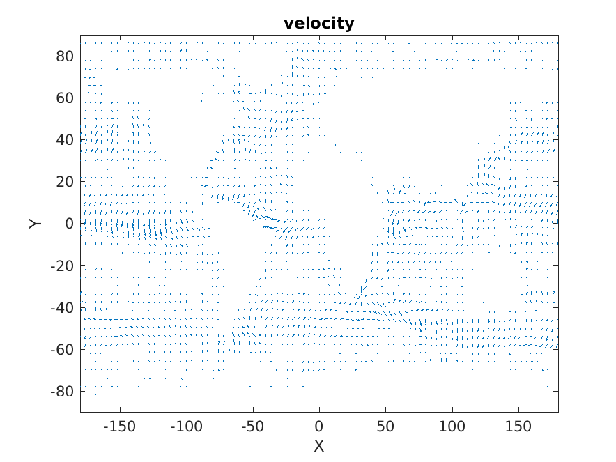
Current velocity quiver plot